零、目标
Deep Dream是谷歌推出的一个有意思的技术。在训练好的CNN上,设定几个参数就可以生成一张图象。具体目标是:
- 了解Deep Dream基本原理
- 掌握实现生成Deep Dream 模型
一、技术原理
在卷积网络中,通常输入的是一张图象,经过若干层的卷积运算,最终输出图像的类别。这期间使用到了图片计算梯度,网络根据梯度不断的调整和学习最佳的参数。但是卷积层究竟学习到了什么,卷积层的参数代表了什么,浅层卷积和深层卷积学习到的内容有哪些区别,这些问题Deep Dream可以解答。
假设输入网络的图像为X,网络输出的各个类别的概率为t(t是一个多维向量,代表了多种类别的概率)。设定t[N]为优化目标,不断的让神经网络去调整输入图像X的像素值,让输出t[N]尽可能的大,最后极大化第N类别的概率得到图片。
关于卷积层究竟学到了什么,只需要最大化卷积层的某一个通道数据就可以了。折输入的图像为X,中间某个卷积层的输出是Y,Y的形状是hwc,其中h为Y的高度,w为Y的宽度,c为通道数。卷积的一个通道就可以代表一种学习到的信息。以某一个通道的平均值作为优化目标,就可以弄清楚这个通道究竟学习到了什么,这也是Deep Dream的基本原理。
二、在TensorFlow中使用
- 导入Inception模型
原始的Deep Dream 模型只需要优化ImageNet 模型卷积层某个通道的激活值就可以。因此,应该先导入ImageNet图像识别模型,这里以 Inception 为例。创建 load_inception.py 文件,输入如下代码:
# 导入基本模块
import numpy as np
import tensorflow as tf

# 创建图和会话
graph = tf.Graph()
sess = tf.InteractiveSession(graph=graph)

# 导入Inception模型
# tensorflow_inception_graph.pb 文件存储了inception的网络结构和对应的数据
model_fn = 'tensorflow_inception_graph.pb'
with tf.gfile.FastGFile(model_fn, 'rb') as f:
    graph_def = tf.GraphDef()
    graph_def.ParseFromString(f.read())


# 导入的时候需要给网络制定一个输入图像,因此定义一个t_input作为占位符
# 需要注意的是,使用的图像数据通常的格式为:(height,width,channel),
# 其中height为图像的像素高度,width为图像的像素宽度,chaneel为图像的通道数,一般使用RGB图像,所以通道数为3
t_input = tf.placeholder(np.float32, name='input')
imagenet_mean = 117.0

# 处理输入图像
# 虽然图像的格式是(height,width,channel),但是Inception模型所需的输入格式是(batch,height,width,channel)
# 这是因为(height,width,channel)只能表示一张图片,但在训练神经网络时往往需要多张图片
# 因此在前面加了一维,让输入的图片符合Inception需要的格式
# 尽管这里一次只需要输入一张图片,但是同样也需要将数据变为Inception所需的格式,只不过这里的batch等于1
# 对图像减去一个像素均值
# 原因是在训练Inception 模型的时候,已经做了减去均值的预处理,因此这里使用同样的方法处理,才能保持输入一致
# t_input-imagenet_mean 减去均值,这里使用的Inception模型减去的是一个固定均值117,所以这里也减去117
# expand_dims 执行加一维操作,从[height,width,channel] 变为[1,height,width,channel]
t_preprocessed = tf.expand_dims(t_input - imagenet_mean, 0)

# 导入模型
tf.import_graph_def(graph_def, {'input': t_preprocessed})

# 找到所有的卷积层
layers = [op.name for op in graph.get_operations() if op.type == 'Conv2D' and 'import/' in op.name]

# 输出卷积层层数
print('Number of layers', len(layers))

# 输出mixed4d_3x3_bottleneck_pre_relu 形状
name = 'mixed4d_3x3_bottleneck_pre_relu'
print('shape of %s: %s' % (name, str(graph.get_tensor_by_name('import/' + name + ':0').get_shape())))
这段代码运行后,会输出卷积层总数是59个
注1:
在输出卷积层“mixed4d_3x3_bottleneck_pre_relu”的形状时,输出的结果是(?,?,?,144),原因是此时还不清楚输入图像的个数以及大小,所以前三维的值不确定
- 生成原始图像
以 mixed4d_3x3_bottleneck_pre_relu 卷积层为例,最大化它的某一个通道的平均值,以达到生成图像的目的。
创建 gen_naive.py 文件,导入Inception模型,导入方法同上节。首先定义保存图片的函数:
def savearray(img_array, img_name):
    scipy.misc.toimage(img_array).save(img_name)
    print('img saved : %s' % img_name)
接着创建程序的主要部分:
# 定义卷积层、通道数,并去除对应的Tensor
name = 'mixed4d_3x3_bottleneck_pre_relu'
# 选择任意的通道,这里是139
channel = 139
# 取出 mixed4d_3x3_bottleneck_pre_relu 卷积层的输出层
layer_output = graph.get_tensor_by_name("import/%s:0" % name)

# 定义原始的图像噪声
# 他是一个形状为(224,224,3)的张量,表示初始化图像优化起点
img_noise = np.random.uniform(size=(224, 224, 3)) + 100.0

# 调用 render_navie 函数渲染
render_naive(layer_output[:, :, :, channel], img_noise, iter_n=20)
最后定义渲染函数
def render_naive(t_obj, img0, iter_n=20, step=1.0):
    ''' 渲染函数 :param t_obj:卷积层某个通道的值 :param img0:初始化图像 :param iter_n:迭代的步数 :param step: :return: '''
    # t_score 是优化目标。他是t_obj的平均值
    # t_score 越大,就说明神经网络卷积层对应的通道的平均激活越大
    t_score = tf.reduce_mean(t_obj)
    # 计算t_score对t_input的梯度
    # 代码的目标是通过调整输入图像 t_input ,来让 t_score 尽可能的大
    # 因此使用体服下降法
    t_grad = tf.gradients(t_score, t_input)[0]

    # 创建新图
    img = img0.copy()
    # 迭代 iter_n 每一步都将梯度应用到图像上
    for i in range(iter_n):
        # 在sess中计算梯度,以及当前的score
        g, score = sess.run([t_grad, t_score], {t_input: img})
        # 对img应用梯度,step可以看作学习率
        g /= g.std() + 1e-8
        img += g * step
        print('score(mean)=%f' % (score))

    savearray(img, 'navie.jpg')
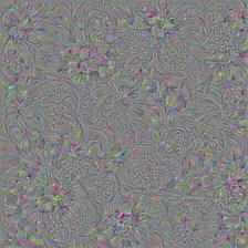
运行程序后,将得到20次迭代后的图像,如下图
- 生成大尺寸图片
上节生成的图片尺寸太小,这节通过代码,将生成的大尺寸的图片。上节中传递图片尺寸的参数是 img_noise ,如果 img_noise 传递更大的值,那么生成的图片尺寸就会更大。但是这样就出现一个问题,生成图片的过程是需要消耗内存/显存的,img_noise 传递的尺寸越大,消耗的内存/显存就越多,最终会因为内存/显存不足,导致渲染失败。如何解决这个问题呢,其实很简单,每次不对整张图片做优化,而是把图片分为几个部分,每次只对一部分做优化,这样消耗的内存/显存就是固定大小的。
新建 gen_multiscale.py 文件,写入如下代码,这个函数可以对任意大小的图像进行提督计算:
def calc_grad_tiled(img, t_grad, title_size=512):
    ''' 对任意大小的图像计算梯度 :param img: :param t_grad: :param title_size:每次优化的大小 :return: '''
    # 每次只对title_size*title_size大小的图像计算梯度
    sz = title_size
    h, w = img.shape[:2]

    # 如果直接计算梯度,在每个 title_size * title_size 的边缘会出现比较明显的边缘效应,影响美观
    # 解决的办法是:生成两个随机数 sx、sy,对图片进行整体移动
    # img_shift 先在行上做整体移动,再在列上做整体移动
    # 防止出现边缘效应
    sx, sy = np.random.randint(sz, size=2)
    img_shift = np.roll(np.roll(img, sx, 1), sy, 0)
    grad = np.zeros_like(img)
    # y,x是开始及位置的像素
    for y in range(0, max(h - sz // 2, sz), sz):
        for x in range(0, max(w - sz // 2, sz), sz):
            # 每次对sub计算梯度。sub的大小是title_size*title_size
            sub = img_shift[y:y + sz, x:x + sz]
            g = sess.run(t_grad, {t_input: sub})
            grad[y:y + sz, x:x + sz] = g

        # 使用np.roll移回去
        return np.roll(np.roll(grad, -sx, 1), -sy, 0)
为了加快图像的收敛速度,可以采用先生成小尺寸,再将图片放大:
# 将图片放大ratio倍
def resize_ratio(img, ratio):
    # 首先确定源像素的范围
    min = img.min()
    max = img.max()
    img = (img - min) / (max - min) * 255
    img = np.float32(scipy.misc.imresize(img, ratio))
    # 使用完 scipy.misc.imresize 函数后,将像素缩放回去
    img = img / 255 * (max - min) + min
    return img

# 生成大尺寸图片
def render_multiscale(t_obj, img0, iter_n=10, step=1.0, octave_n=3, octave_scale=1.4):
    ''' 生成大尺寸图片 :param t_obj: :param img0: :param iter_n: :param step: :param octave_n:放大次数 :param octave_scale:放大倍数 :return: '''
    # 同样定义目标梯度
    t_score = tf.reduce_mean(t_obj)
    t_grad = tf.gradients(t_score, t_input)[0]

    img = img0.copy()
    # 先生成小尺寸图像
    # 然后调用 resize_ratio 将小尺寸图像放大 octave_scale 倍
    # 再使用放大后的图像作为初始值进行计算
    for octave in range(octave_n):
        if octave > 0:
            # 每次将图片放大octave_scale倍
            # 共放大octave_n-1次
            img = resize_ratio(img, octave_scale)
        for i in range(iter_n):
            # 计算任意大小图像的梯度
            g = calc_grad_tiled(img, t_grad)
            g /= g.std() + 1e-8
            img += g * step
            print('.', end=' ')
    savearray(img, 'multiscale.jpg')
下面编写主内容
if __name__ == '__main__':
    name = 'mixed4d_3x3_bottleneck_pre_relu'
    channel = 139
    img_noise = np.random.uniform(size=(224, 224, 3)) + 100.0
    layer_output = graph.get_tensor_by_name("import/%s:0" % name)
    render_multiscale(layer_output[:, :, :, channel], img_noise, iter_n=20)
运行代码后,将生成一张大尺寸的图片,如下图:
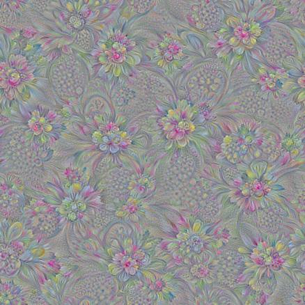
从图中可以看出,mixed4d_3x3_bottleneck_pre_relu 卷积层的第139个通道实际上就是学到了某种花朵的特征。
- 生成高质量图片
前面两节生成的图片都是分辨率不高的图片,这节将生成高质量的图片。在图像处理算法中,有 高频成分 和 低频成分 之分。所谓高频成分,是指图像中灰度、颜色、明度变化比较剧烈的地方,比如边缘、细节部分。低频成分是指图像变化不大的地方,比如大块色块、整体风格。
上节生成的图片高频成分太多,图片不够柔和。如何解决这个问题呢?一种方法是针对高频成分加入损失,这样图像在生成的时候就会因为新加入损失的作用二发生变化,但是加入损失会导致计算量和收敛步数增大。另一种方法是 放大低频梯度 ,对梯度进行分解,降至分为 高频梯度 和 低频梯度 ,在人为的去放大低频梯度,就可以得到较为柔和的图像。
一般情况下,要使用 拉普拉斯金字塔 对图像进行分解,这种算法可以把图片分解为多层。同时,也可以对梯队进行分解,分解之后,对高频的梯度和低频的梯度都做标准化,可以让梯度的低频成分和高频成分差不多,表现在图像上就会增加图像的低频成分,从而提高生成图像的质量。这种方法称为 拉普拉斯金字塔标准化,具体实现代码如下:
k = np.float32([1, 4, 6, 4, 1])
k = np.outer(k, k)
k5x5 = k[:, :, None, None] / k.sum() * np.eye(3, dtype=np.float32)

# 这个函数将图像分为低频和高频成分
def lap_split(img):
    with tf.name_scope('split'):
        # 做一次卷积相当于一次平滑,因此lo为低频成分
        lo = tf.nn.conv2d(img, k5x5, [1, 2, 2, 1], 'SAME')
        # 低频成分缩放到原始图像大叫就得到lo2,再用原始图像img减去lo2,就得到高频成分hi
        lo2 = tf.nn.conv2d_transpose(lo, k5x5 * 4, tf.shape(img), [1, 2, 2, 1])
        hi = img - lo2
    return lo, hi


# 这个函数将图像img分成n层拉普拉斯金字塔
def lap_split_n(img, n):
    levels = []
    for i in range(n):
        # 调用lap_split将图像分为低频和高频部分
        # 高频部分保存到levels中
        # 低频部分再继续分解
        img, hi = lap_split(img)
        levels.append(hi)
    levels.append(img)
    return levels[::-1]


# 将拉普拉斯金字塔还原到原始图像
def lap_merge(levels):
    img = levels[0]
    for hi in levels[1:]:
        with tf.name_scope('merge'):
            img = tf.nn.conv2d_transpose(img, k5x5 * 4, tf.shape(hi), [1, 2, 2, 1]) + hi
    return img


# 对img做标准化
def normalize_std(img, eps=1e-10):
    with tf.name_scope('normalize'):
        std = tf.sqrt(tf.reduce_mean(tf.square(img)))
        return img / tf.maximum(std, eps)


# 拉普拉斯金字塔标准化
def lap_normalize(img, scale_n=4):
    img = tf.expand_dims(img, 0)
    tlevels = lap_split_n(img, scale_n)
    # 每一层都做一个normalize_std
    tlevels = list(map(normalize_std, tlevels))
    out = lap_merge(tlevels)
    return out[0, :, :, :]
编写完拉普拉斯标准化函数后,现在编写生成图像的代码:
# 将一个Tensor函数转换成numpy.ndarray 函数
def tffunc(*argtypes):
    placeholders = list(map(tf.placeholder, argtypes))

    def wrap(f):
        out = f(*placeholders)

        def wrapper(*args, **kw):
            return out.eval(dict(zip(placeholders, args)), session=kw.get('session'))

        return wrapper

    return wrap


def render_lapnorm(t_obj, img0,
                   iter_n=10, step=1.0, octave_n=3, octave_scale=1.4, lap_n=4):
    # 同样定义目标和梯度
    t_score = tf.reduce_mean(t_obj)
    t_grad = tf.gradients(t_score, t_input)[0]
    # 将lap_normalize转换为正常函数
    lap_norm_func = tffunc(np.float32)(partial(lap_normalize, scale_n=lap_n))

    img = img0.copy()
    for octave in range(octave_n):
        if octave > 0:
            img = resize_ratio(img, octave_scale)
        for i in range(iter_n):
            g = calc_grad_tiled(img, t_grad)
            # 唯一的区别在于我们使用lap_norm_func来标准化g!
            g = lap_norm_func(g)
            img += g * step
            print('.', end=' ')
    savearray(img, 'lapnorm.jpg')

if __name__ == '__main__':
    name = 'mixed4d_3x3_bottleneck_pre_relu'
    channel = 139
    img_noise = np.random.uniform(size=(224, 224, 3)) + 100.0
    layer_output = graph.get_tensor_by_name('import/%s:0' % name)
    render_lapnorm(layer_output[:, :, :, channel], img_noise, iter_n=20)
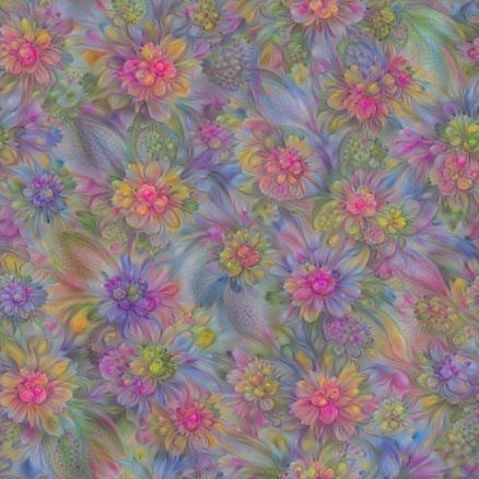
运行上面代码后,将生成高质量的图片:
- 生成最终的图片
前面已经讲解了如何通过极大化卷积层摸个通道的平均值生成图片,并学习了如何生成更大和质量更高的图像。但是最终的Deep Dream 模型还需要对图片添加一个背景。具体代码如下:
def resize(img, hw):
    min = img.min()
    max = img.max()
    img = (img - min) / (max - min) * 255
    img = np.float32(scipy.misc.imresize(img, hw))
    img = img / 255 * (max - min) + min
    return img


def render_deepdream(t_obj, img0, iter_n=10, step=1.5, octave_n=4, octave_scale=1.4):
    t_score = tf.reduce_mean(t_obj)
    t_grad = tf.gradients(t_score, t_input)[0]

    img = img0
    # 同样将图像进行金字塔分解
    # 提取高频和低频的方法比较简单,直接缩放
    octaves = []
    for i in range(octave_n - 1):
        hw = img.shape[:2]
        lo = resize(img, np.int32(np.float32(hw) / octave_scale))
        hi = img - resize(lo, hw)
        img = lo
        octaves.append(hi)

    # 先生成低频的图像,再依次放大并加上高频
    for octave in range(octave_n):
        if octave > 0:
            hi = octaves[-octave]
            img = resize(img, hi.shape[:2]) + hi
        for i in range(iter_n):
            g = calc_grad_tiled(img, t_grad)
            img += g * (step / (np.abs(g).mean() + 1e-7))
            print('.', end=' ')

    img = img.clip(0, 255)
    savearray(img, 'deepdream.jpg')


if __name__ == '__main__':
    img0 = PIL.Image.open('test.jpg')
    img0 = np.float32(img0)

    # name = 'mixed4d_3x3_bottleneck_pre_relu'
    name = 'mixed4c'
    # channel = 139
    layer_output = graph.get_tensor_by_name('import/%s:0' % name)
    # render_deepdream(layer_output[:, :, :, channel], img0, iter_n=150)
    render_deepdream(tf.square(layer_output), img0)